corona26
Guide Method Prediction Simulation GitHub

Can I predict an eclipse corona from a real magnetic field?

On 12 August 2026 the Moon removes the Sun for 37 seconds over Colmenar Viejo, north of Madrid. Today the Sun’s magnetic field has already been measured. This is an attempt to cross the gap between those two facts, and then find out — by looking up — how badly it went.

A potential-field reconstruction of the coronal magnetic field, a topology-informed electron-density model, and an exact Thomson-scattering renderer. Not a thermodynamic MHD model, and it does not pretend to be one. Every approximation is written down and ranked by risk.

  • Totality observed 2026-08-12
  • Boundary condition 2026-08-11 04:00 UTC
  • Ensemble 60 members
  • Phase Validation underway

// field guide

A practical guide for Colmenar Viejo

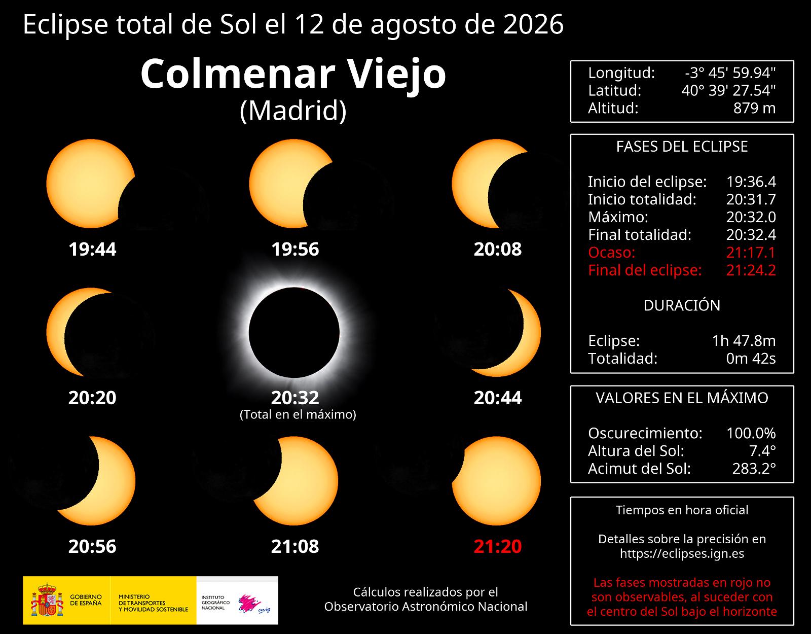
The Sun will be very low: 7.4° altitude at azimuth 283.2°, toward west-northwest (WNW). A clear horizon matters more than gaining a few metres of proximity: buildings, trees and the Guadarrama range can hide totality.

Eye safety: do not improvise

Use trustworthy ISO 12312-2 solar viewers throughout every partial phase. Remove them only after ALL of the photosphere has disappeared; replace them as soon as the first bright point appears and, if in any doubt, before C3. Ordinary sunglasses and homemade filters are not safe.

Cameras, binoculars and telescopes need a purpose-made solar filter secured in front of the objective. Eclipse glasses behind concentrating optics are dangerous. If you are improvising, do not handle magnifying optics during transitions: observe unaided with the correct viewer.

Local timetable (CEST)

OAN/IGN circumstances for Colmenar Viejo
First contact (C1)19:36:24
Totality begins (C2)20:31:42
Maximum20:32:00
Totality ends (C3)20:32:24
Sunset21:17:06

Totality lasts about 37–42 seconds, depending on the exact location and calculation model. It is not universal across Colmenar Viejo, and a clock never replaces checking that the photosphere has disappeared.

Before leaving

  • Check for a clear view toward 283° WNW and arrive early.
  • Inspect viewers; discard scratched, punctured or damaged ones.
  • Bring water, a charged battery and a safe location away from traffic.
  • Secure every objective filter before pointing equipment at the Sun.
  • Avoid dry grass and any heat source or fire risk.

A 37–42 second script

  1. Prepare and start recording before C2. Experience > phone: do not spend totality configuring a camera.
  2. First seconds: notice the chromosphere, red prominences and inner corona.
  3. Middle: take in the corona's overall shape, then the landscape and horizon.
  4. Last 8–10 s: viewers in hand; put them on before C3 if there is any doubt.

If there are clouds

Keep viewers on throughout partial phases and observe ambient light, temperature, the horizon and animal behaviour. A cloud is never a solar filter, even when the Sun looks dim.

What to notice, and why it happens

During partial phases, gaps between leaves act as pinhole cameras and project crescents; shadows sharpen and the light loses saturation, sometimes appearing metallic. Near totality, shadow bands may appear: moving patterns produced by atmospheric turbulence, subtle and not guaranteed.

At the contacts, lunar valleys pass points of photospheric light: Baily's beads. The last or first bright point beside the corona forms the diamond ring. The chromosphere and prominences look red because of strong hydrogen emission; the lunar disk looks black because its night side blocks a vastly brighter photosphere.

The corona looks white because free electrons Thomson-scatter the full mixture of photospheric light without selecting one dominant visible colour. The sky does not become full night: outside the narrow umbra, the atmosphere and peripheral horizon remain illuminated, producing 360° twilight. The umbra may be visible approaching or departing across the landscape.

At only 7.4°, light crosses much more atmosphere: aerosols, humidity and haze increase extinction and reduce contrast and colour, making the WNW horizon critical. Venus is plausible, but do not sacrifice the corona searching for it. Cooling, wind and animal responses vary greatly and may be confused with sunset; they are worthwhile observations, not guarantees.

Official and safety sources

// method

Five stages, each with a stated approximation

The corona is visible during totality because free electrons scatter photospheric light. Its shape is set almost entirely by the magnetic field. So the chain runs from a measured surface field to a synthetic image, and every link introduces error worth naming.

  1. Photospheric magnetic field ADAPT-GONG global map, 12 realisations. The far side is modelled, not observed.
  2. Coronal field by PFSS Solve ∇²Φ = 0 between the surface and a source surface. Current-free, static, and the source surface is fictional.
  3. Magnetic topology Trace field lines; open ones become coronal holes, closed ones become streamers. Exact, given the field.
  4. Electron density An empirical radial profile modulated by topology. A proxy. This is the weakest link and it is labelled as such.
  5. Thomson scattering Integrate along every line of sight with the van de Hulst kernel. Genuinely exact: the corona is optically thin, τ ≈ 10⁻⁶.

what this is not

Predictive Science run a time-dependent MHD model for this eclipse, assimilating far-side magnetograms from Solar Orbiter/PHI. They will be better than this. That is the point of having them as a baseline — the interesting question is where a cheap model breaks, and by how much.

// phase A — complete

The uncertainty is not where you would guess

The dominant error in this whole pipeline is not the renderer and not even PFSS. It is that we cannot see the far side of the Sun. Global maps reconstruct the hidden hemisphere with a surface flux-transport model, and August 2026 is near solar maximum, when active regions evolve in days.

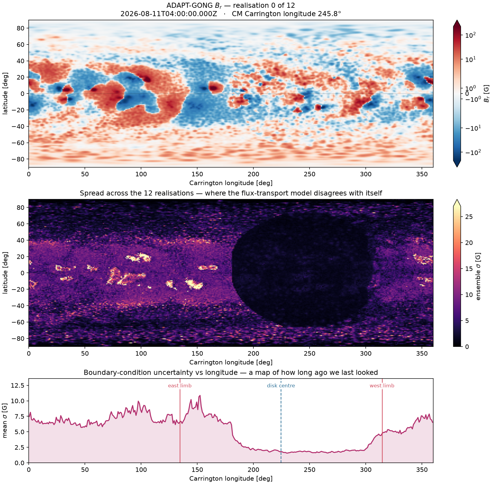
ADAPT ships twelve realisations of that reconstruction. They agree almost exactly on how much flux exists — total unsigned flux varies by only 1.14%. They disagree sharply on where it is, and the disagreement is organised by longitude.

Three panels: the ADAPT-GONG radial magnetic field, the spread across its twelve realisations, and that spread averaged as a function of Carrington longitude
The boundary condition and its own error bar. Bottom panel: ensemble spread against longitude is effectively a map of how long ago each part of the Sun was last observed.
Ensemble spread at totality, when the disk centre sits at Carrington longitude 224.5°
RegionCarrington longitudeSpread
Disk centre224.5°1.85 G
West limb314.5°4.11 G
East limb134.5°7.71 G

The east limb is the edge that most recently rotated out of the far side, so it is the longest unobserved. It carries 4.2× the uncertainty of disk centre — and on an eclipse image the limbs are exactly where the structure lives, because streamers are seen edge-on against the sky.

a pre-registered prediction about our own failure

The preregistered prediction states that, if this model fails, it should fail asymmetrically, worse on the east limb. If it fails symmetrically, the far-side field was not the limiting factor and something else is — the source surface, or the density proxy. Either way we learn something, which is more than a confident picture would have given us.

// phase B — complete

A parameter nobody has measured

PFSS assumes the corona carries no currents, so the field is the gradient of a potential satisfying Laplace’s equation. The model’s real physical content is its upper boundary: a source surface at radius Rss where the field is forced radial, standing in for the solar wind dragging it open.

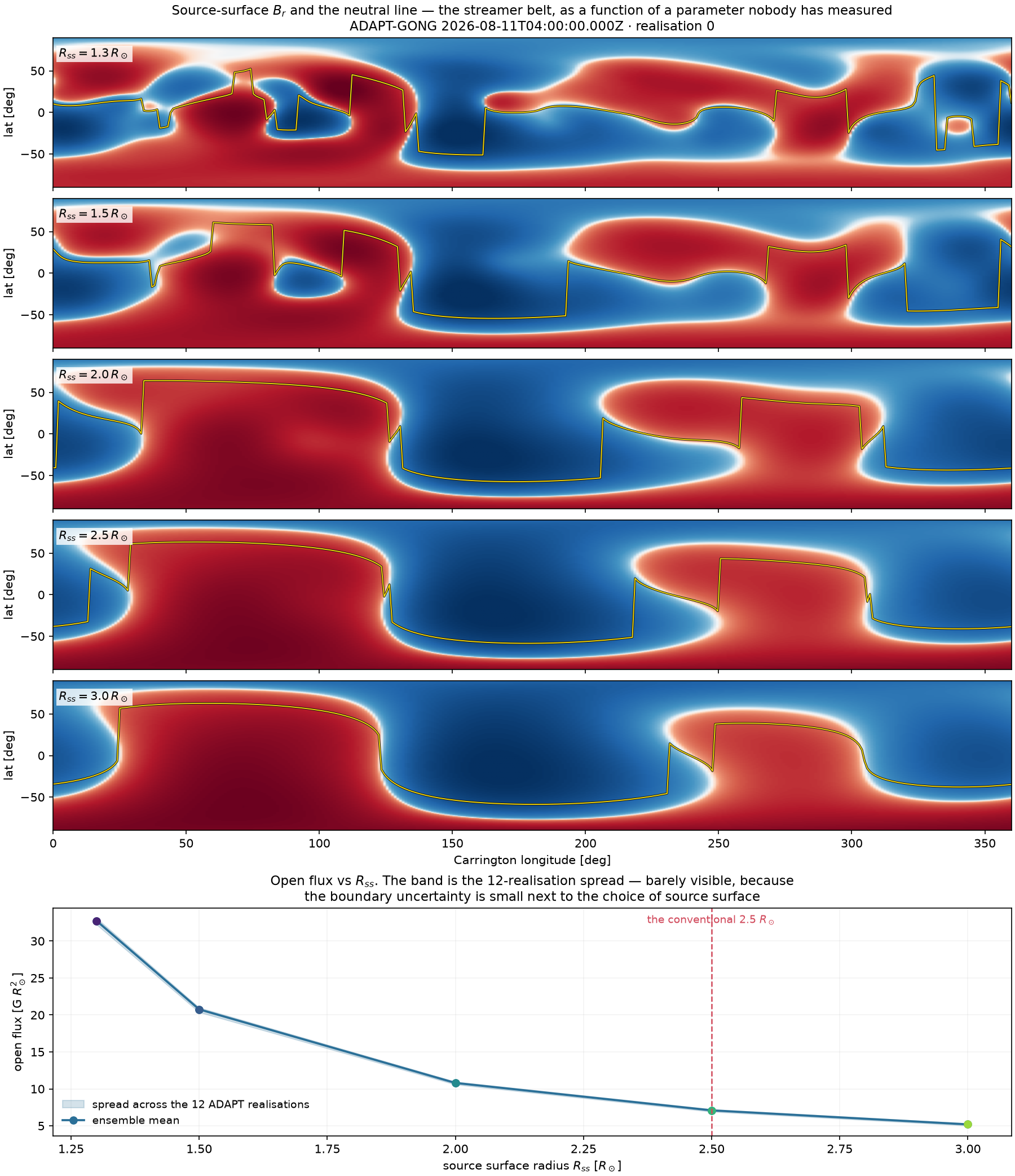
There is no such surface. Rss = 2.5 R is a convention from 1969, and recent work benchmarking against eclipse images finds the best value moves with the solar cycle. So we do not pick one — we run five, across all twelve realisations. Sixty solves, 124 seconds on a laptop.

Before trusting any of it: for a pure dipole boundary the potential has a closed form, and the solver must reproduce it.

Br(r, θ) = b₀ cosθ · (Rss⁻³ + 2r⁻³) / (2 + Rss⁻³)

It does, to 5% at the source surface, with the polarity the right way round, and it reproduces the input boundary map to 0.03% RMS. Sign conventions, normalisation and the upper boundary condition are all pinned by that single test.
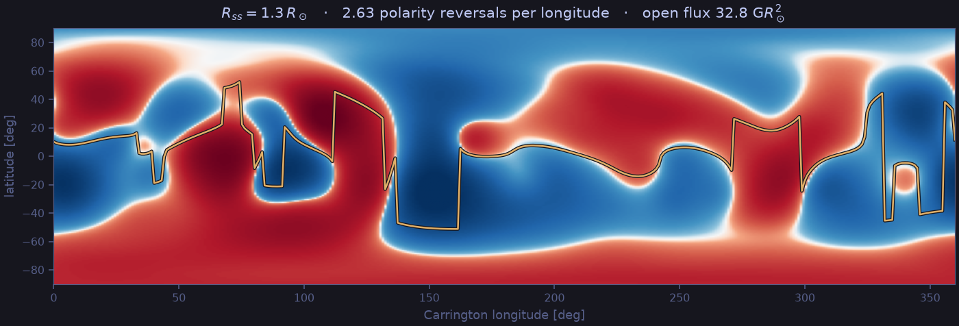
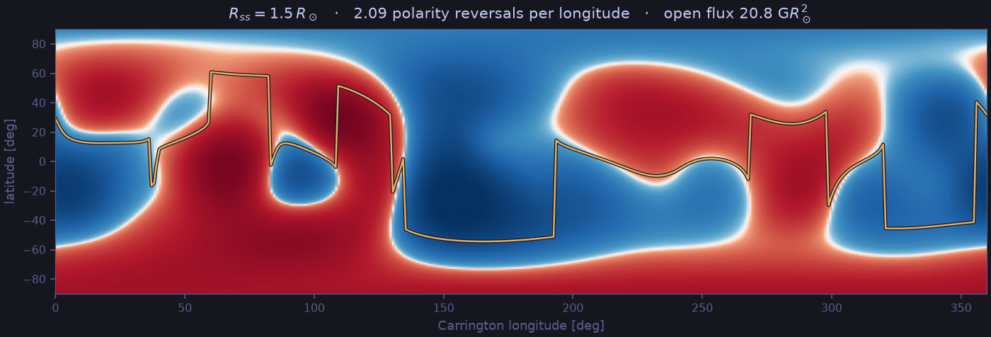
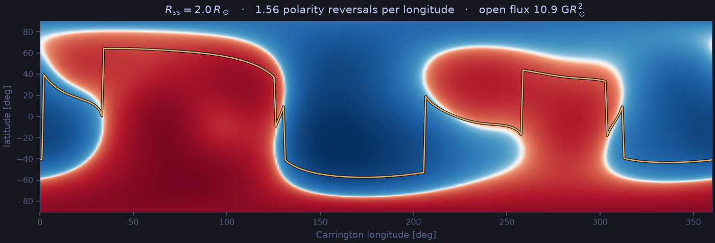
Five source-surface radial field maps with their neutral lines, from 1.3 to 3.0 solar radii, plus open flux against source surface radius
The same Sun, five source surfaces. The yellow line is the neutral line — the base of the heliospheric current sheet, where the streamer belt sits.

// phase C — complete

Where the wind escapes, and where plasma stays trapped

With the field solved, field lines are integrated from 16,200 equal-area photospheric seeds and classified. Closed lines return to the surface at both ends: they trap plasma, are overdense, and build the streamers. Open lines reach the source surface: plasma escapes as solar wind, the region is underdense, and it forms a coronal hole — dark in white light.

That classification is what turns a magnetic field into something we can put a density on, so it feeds directly into Phase D.

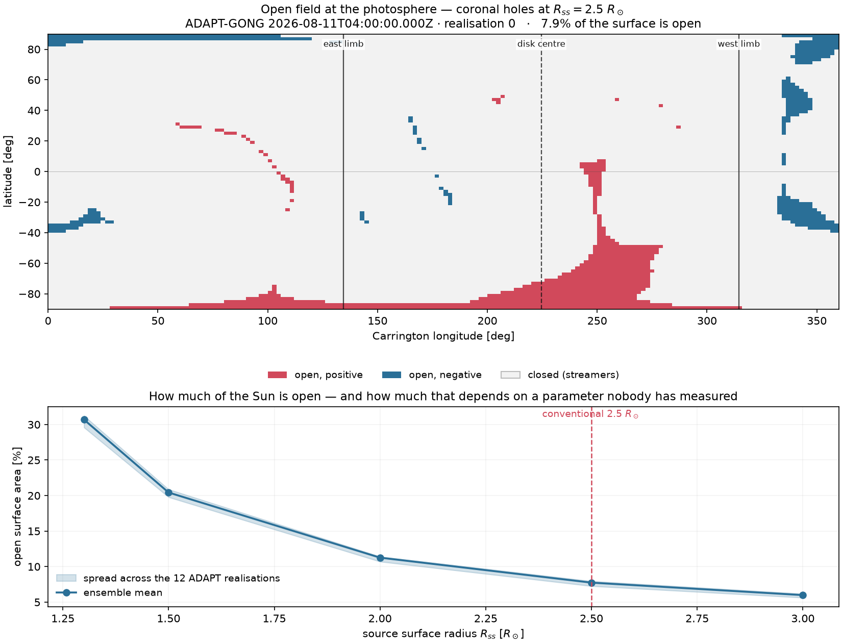
Map of open magnetic field at the photosphere showing coronal holes by polarity, and open surface area against source surface radius
Coronal holes, and how much of the Sun is open. A large positive south-polar hole extends to the equator near longitude 250°, close to disk centre at totality.

The classification is converged: doubling the integration step budget changes zero seeds. That matters, because a line that exhausts its budget mid-flight is indistinguishable from one that escaped.

Open solar surface area, mean over the 12-realisation ensemble
RssOpen areaBoundary spread
1.3 R30.69%1.64 pp
1.5 R20.43%1.10 pp
2.0 R11.26%0.72 pp
2.5 R7.74%0.70 pp
3.0 R5.99%0.56 pp

this ratio is a clean one

Open area varies 26× more across source surfaces (24.7 percentage points) than across boundary realisations (0.94 pp). Unlike open flux, nothing here is definitional: open area is always measured at the photosphere, a fixed radius, while the parameter being varied lives far above it. Choosing Rss = 2.5 instead of 1.5 changes how much of the Sun is open from 20% to 8%.

// phases D and E — complete

The prediction

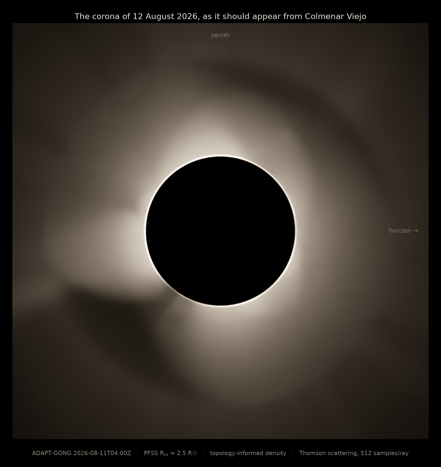
This is what the model, written before totality, predicted for a field north of Madrid on 12 August 2026 at 20:31 CEST. Zenith is up, so this is the orientation the eye sees, not the solar-north-up convention: solar north is tilted 34.7° from vertical.

The predicted white-light corona of the 12 August 2026 eclipse, a bright inner ring with streamer lobes and dark coronal hole wedges, oriented as seen from Colmenar Viejo
The corona of 12 August 2026, predicted from the previous day's magnetic field. The bright lobes are streamers — plasma trapped on closed field. The dark wedges are coronal holes, where the solar wind escapes.

The test that pins everything at once

The Sun is not a point source — an electron at 1.5 R sees a disk 42° wide — so the scattering angle varies across the disk and must be integrated over it with limb darkening. Van de Hulst did that integral in 1950, leaving four closed-form coefficients. The decisive test is that far from the Sun the full finite-disk kernel must collapse onto the textbook dipole pattern:

B(χ) / B(90°)  →  1 + cos²(χ)      as r → ∞

It does, to 0.2%. That single check pins the sign, the normalisation and the whole disk integral at once — nothing else in the kernel can be wrong while it passes.

Final render cost and checks
Kernel evaluations415M per frame
Render time118 s (NumPy, CPU)
Field lines traced884k
Quadrature convergence0.98% worst case
Peak memory1.8 GB

what is honest here and what is not

The geometry is real: observer position, solar orientation, scattering angles, the occulting disk. The scattering is exact. The magnetic topology is a genuine PFSS solution from a real magnetogram.

The density is a proxy — closed field 3.5× enhanced, open field 0.4× depleted, over a Baumbach–Allen radial profile. Those are knobs, fixed before any comparison with Predictive Science so we cannot tune our way into agreement.

And the structure is too smooth. Real coronae show fine radial striations; a potential field with a two-valued density proxy cannot produce them. If the observed corona is sharper and more filamentary than this, that is the density model failing, not the renderer.

// simulation

Move the source surface yourself

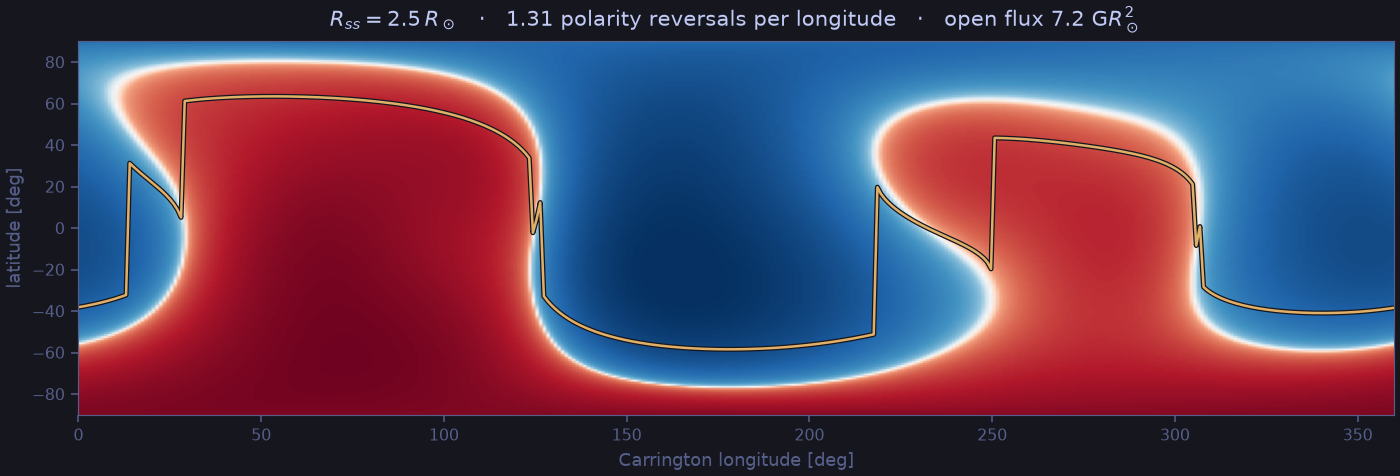
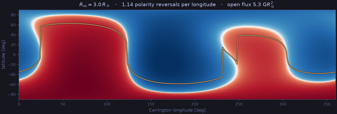
These are not the same picture at different scales. As Rss falls, the belt stops being a single band and breaks into several distinct streamers. These predict visibly different eclipses.

Source-surface radial field and neutral line for a source surface at 2.5 solar radii
Rss = 2.5 R — 1.31 polarity reversals per longitude, open flux 7.2 G R2. The conventional choice since Altschuler & Newkirk (1969). One dominant belt with a couple of excursions.

ADAPT-GONG 2026-08-11T04:00Z · realisation 0 · nr = 100

Which uncertainty wins, stated carefully

Open flux varies 48× more across the five source surfaces than across the twelve boundary realisations. We are not going to lead with that number: open flux is measured at the source surface, whose radius is the parameter being varied, so part of that ratio is definitional rather than physical.

The honest metric is the one an eclipse actually shows: where the streamer belt sits on the sky.

RMS scatter in neutral-line latitude
Across 12 ADAPT realisations, fixed Rss5.3°
Across 5 source surfaces, fixed realisation20.5°
Ratio3.8×

So the ranking survives with a corrected magnitude. The source-surface choice moves the streamer belt about four times as much as the entire far-side uncertainty, not fifty. Both matter; the fictional parameter matters more.

// post-eclipse check

General shape partially supported

provisional · qualitative only

Six frames from the official ESA/Javalambre telescope feed, between 01:03:50 and 01:04:40, consistently show a non-circular, multipolar corona with roughly 3–4 broad fans and a visual extent of ~2–2.5 R. That coarse morphology is compatible with the frozen prediction, but it is not an official score.

Qualitative matches

  • Multipolar character rather than a uniform circular corona.
  • Roughly 3–4 broad coronal sectors.
  • Comparable visual radial extent.
  • The coarse structure remains stable across feed exposures.

Visible discrepancies

  • The real corona is more filamentary and abrupt.
  • Brightness is more concentrated and less balanced.
  • The model's density proxy is too smooth.
  • The model does not predict prominences.

Why it cannot be scored yet

The available feed is compressed 1920×1080 video and does not document solar north, optical parity or calibration. It therefore cannot support position-angle (PA) matching, test the preregistered east-west asymmetry, or rigorously measure radial extent. Its status is qualitative_only; the official score remains pending.

Primary-observation candidate status, as of 12 Aug 2026 21:34 CEST
SourceAvailable provenanceOfficial-score blocker
Commons · Logroño 3000×4000 JPEG; EXIF 18:28:20 UTC; GPS; CC BY-SA 3.0. CustomRendered; optical chain, parity and coverage to 2.5 R cannot be certified.
IGN/OAN · Yebes Institutional Solar Tower, white light. Stream without RAW/FITS, orientation or calibration.
IAC/NATE Institutional observing programme. No suitable public originals yet.

official_candidate: none_available

The official validation protocol requires selecting an observation by provenance before comparing its morphology. Waiting for better data protects the result from choosing, after inspection, whichever image most favours the prediction.

Reproducibility note

The qualitative check used six frames distributed from 01:03:50 to 01:04:40 in the linked feed. No third-party images are embedded, and these frames were not used to run the official protocol.

the prediction remains prior

The prediction and its source magnetogram were published before totality, with the input observation time recorded. This later check does not modify those artefacts or their history.